Propagation of Errors in calculations
Level 1 (gold) - this material needs some prerequisites that are covered in the first year mathematics for chemists course. These are Taylor expansions, partial differentiation, and functions of several variables.
This section applies statistical methods to work out how errors in measured quantities affect the results of calculations. A related question is: how does uncertainty in the conditions affect a measurement (for example how do fluctuations in the temperature affect a rate constant measurement)?
Suppose y and x are related through y = f(x). A measurement X of the quantity x is made, but the value of y is required. A simple example might be the calculation of the volume of a cube after measuring one of its sides, or the calculation of the equilibrium constant for an isomerisation reaction from a measurement of the proportion of starting material isomerised at equilibrium.
We assume that the true values obey the equation; in statistical terms the true values are the means of the underlying distributions.
![]()
of course this may not be true, a real statistician would want to know how the function transforms the underlying distribution to give a new distribution for Y, however if the distributions are narrow this is not a bad starting point.
The problem is that we do not know mx, we only know an experimental estimate of it, X. So we make an estimate of y, Y, from Y = f(X).
Now X - mx = DX (the deviation of X from the theoretical mean), and similarly Y - my = DY. Hence
![]()
Now we take a Taylor expansion of the function f about the true value,
![]()
and cancel the true values,
giving
![]()
This is an equation that tells us how the actual error in the measured x translates through the function to y.
The situation is particularly simple if the Taylor expansion can be truncated after the first correction term.
The problem is that we do not know the actual error in x, but we can estimate its variance, which is the expectation of the squared error. So squaring and taking expectations (see previous tutorial),

and finally taking the square root we get a simple relationship between the standard deviation of x and the standard deviation of y:

Although we have proved this relationship for the true (underlying) standard deviations we assume that it also applies to the estimated standard deviations. (It does to this first order approximation.) Remember that we have truncated the Taylor series after one term, and so this procedure will only work if the standard deviations are small enough that this truncation is a good approximation.
A spherical water droplet has a radius measured to be 3.00 mm with an estimated standard deviation of 0.03 mm. Calculate its volume and estimate the error.
The volume is 4pr3/3 = 1.131x10⁻¹⁶ m3.
Using the propagation of errors formula

which has the value 3.4x10⁻¹⁸ m3.
Note that the 1% error in r has become a 3% error in V, in line with our rule of thumb.
How is a rate constant affected by random errors in the temperature?
The temperature dependence of a rate constant is given by the Arrhenius equation:
![]()
where A, E and R are all constant for a reaction.
Applying the propagation of error formula

which can also be rewritten in a convenient form using relative errors:
![]()
Example 3 - Equilibrium constant
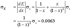
In a keto-enol equilibrium measurement the fraction of enol at equilibrium is found to be 0.200 with a standard deviation of 0.004. Calculate the equilibrium constant and estimate the error in it.
The fraction of the keto form is 0.800, so the equilibrium constant is
![]()
Using the propagation of errors formula

In many calculations several measured quantities need to be combined together with their respective errors. The method is essentially the same for one variable, but requires partial derivatives.
Suppose z = f(x,y), which we interpret to refer to the true mean values. But we measure values X and Y and use the function to infer Z = f(X,Y).
Using X = mx + DX, the true value plus the deviation of the measured value from the true value, and similar equations for Y and Z we get
![]()
As before, expand as a Taylor series in the two variables and cancel the true values

linking the actual errors in the measurements to the error in the result.
Since we do not know the actual errors, but can estimate the standard deviations, we square and take expectations:

If the measurements of X and Y are independent the covariance is zero and the cross term may be omitted.
Example 4 - molar conductivity
How does the error in the molar conductivity depend on errors in the electrolytic conductivity and the concentration of the solution?
The basic equation is L = k / c. Hence

which can also be written in terms of relative errors

Since it is likely that errors in electrolytic conductivity and concentration are positively correlated it is probably not justifiable to neglect the covariance term. However, in this case neglect of the covariance will lead to an overestimate of the error in the result and so is at least safe.