Level 0 (green)- this is basic material that you have probably encountered already, although the approach may be slightly different. No prior knowledge is assumed. The section on unbiased estimators is more advanced, but still requires no prior knowledge.
Measurements are not perfectly repeatable, but tend to cluster in some observed range.
The underlying distribution is a theoretical concept that describes the probability distribution (or density) for the value of the measurement. Typically, for a measurement X that can take a value in a continuous range,
![]()
The aim of statistics is to extract information about the underlying distribution from a finite number of measurements. It is obviously difficult to extract the whole distribution, unless it has a known form with a small number of parameters. However, it is possible to define parameters that characterise the distribution in some way and to estimate these from the data.
The most commonly used parameter is the theoretical mean, which is calculated formally from the underlying density by an integral, which has to cover the whole space available for the measurement.
![]()
Parameters obtained by this type of integral are called expectations, and the shorthand
m = E(X) is sometimes used, which can be read m is the expectation value of X.
Although the expectation is a theoretical construction, it can be thought of as the limiting average of the required quantity over an infinitely large sample.
In the same way a theoretical standard deviation s can be defined to describe the width of the underlying distribution:
![]()
The formula for the variance can be written in an alternative form, which is often convenient:
![]()
this can be shown by expanding the square using the binomial theorem and recognising that E[X]=m.
Note that the bracket can be expanded because expectation is a linear operator (if in doubt just substitute in the integral).
In many cases more than one quantity may be measured, and it is important to know whether the value of one variable has any effect on the other. For example two measurements of the same quantity by different students should be independent of one another, since the value obtained by one does not affect the value obtained by the other. However, in an experiment where two rate constants are determined in the same system, the values may not be independent because the main source of error will be temperature fluctuations, which affect the two rate constants in the same way.
The correlation of two quantities in the theoretical distribution may be measured using the covariance, defined by
![]()
as for the variance, the second form follows simply by multiplying the bracket out and identifying the means when they occur.
If two variables are independent their covariance is zero.
If the covariance is positive then a large value of one will tend to be associated with a large value of the other.
If the covariance is negative then a large value of one will tend to be associated with a small value of the other.
Sometimes the correlation is measured using a dimensionless parameter called the correlation coefficient
r = sXY / sX sY
If X and Y are independent calculate the variance of X + Y.

Since the covariance is zero the middle term can be dropped.
The reason that this is an important example is that in an idealised experiment repeated measurements are independent of one another and so for such an experiment the variance of the sum is equal to the sum of the variances.
And this result generalises immediately to the sum of any number of independent measurements.
If N independent measurements are made of the same quantity by the same method they will all have the same undelying distribution (including mean and standard deviation).
Then the sum of the measurements will have variance Ns2, because it will be a sum of N identical terms, all equal to s2.
An important consequence of this result is for the variance of the sample mean.
The sample mean is simply the sum of the measurements divided by N.
Therefore the variance of the sample mean will be the variance of the sum divided by N2.

This supplies the proof that the standard error of the mean is a factor√Nsmaller than the standard deviation of a single measurement as claimed in the section on standard error.
A statistic is a quantity calculated from the data that estimates some parameter of the underlying distribution. For example the mean or the variance.
It is desirable that following a long run of experiments the statistic should home in on the correct value of the required parameter. Another way to say this is that the expectation of the statistic should equal the correct value. Such a statistic is called an unbiased estimator.
Example of an unbiased estimator - the sample mean
The sample mean is defined by

The expectation of this quantity is

The sample mean is therefore an unbiased estimator of the theoretical mean.
Example - estimating the theoretical variance
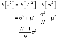
If we want to try to estimate the variance of the unerlying distribution the obvious place to start is the sample variance,

To find the expectation of this quantity we need to know
![]()
which follows from the definition of the variance.
We also need to know

which follows because the mean of m is m and the variance of m is s2/N as proved in the section on covariance.

Hence, the sample variance underestimates the true variance by a factor (N-1)/N, and the form

is an unbiased estimator of the true variance, as discussed earlier.